Root mean square

In mathematics, the root mean square (abbreviated RMS or rms), also known as the quadratic mean, is a statistical measure of the magnitude of a varying quantity. It is especially useful when variates are positive and negative, e.g., sinusoids. RMS is used in various fields, including electrical engineering.

It can be calculated for a series of discrete values or for a continuously varying function. The name comes from the fact that it is the square root of the mean of the squares of the values. It is a special case of the generalized mean with the exponent p = 2.

1 Definition
2 RMS of common waveforms
3 Uses
4 RMS in frequency domain
5 Relationship to the arithmetic mean and the standard deviation
6 See also
7 References
8 External links

Definition

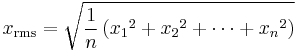
The RMS value of a set of values (or a continuous-time waveform) is the square root of the arithmetic mean (average) of the squares of the original values (or the square of the function that defines the continuous waveform).

In the case of a set of $n$ values $\{x_1,x_2,\dots,x_n\}$ , the RMS value is given by:

$x_{\mathrm{rms}} = \sqrt {\frac{1}{n}\left({{x_1}^2 %2B {x_2}^2 %2B \cdots %2B {x_n}^2}\right)}$

The corresponding formula for a continuous function (or waveform) $f(t)$ defined over the interval $T_1 \le t \le T_2$ is

$f_{\mathrm{rms}} = \sqrt {{1 \over {T_2-T_1}} {\int_{T_1}^{T_2} {[f(t)]}^2\, dt}},$

and the RMS for a function over all time is

$f_\mathrm{rms} = \lim_{T\rightarrow \infty} \sqrt {{1 \over {2T}} {\int_{-T}^{T} {[f(t)]}^2\, dt}}.$

The RMS over all time of a periodic function is equal to the RMS of one period of the function. The RMS value of a continuous function or signal can be approximated by taking the RMS of a series of equally spaced samples. Additionally, the RMS value of various waveforms can also be determined without calculus, as shown by Cartwright.^[1]

In the case of the RMS statistic of a random process, the expected value is used instead of the mean.

RMS of common waveforms

Waveform	Equation	RMS
DC, constant	$y=a\,$	$a\,$
Sine wave	$y=a\sin(2\pi ft)\,$	$\frac{a}{\sqrt{2}}$
Square wave	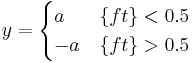$y=\begin{cases}a & \{ft\} < 0.5 \\ -a & \{ft\} > 0.5 \end{cases}$	$a\,$
Modified square wave	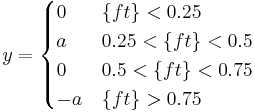$y=\begin{cases}0 & \{ft\} < 0.25 \\ a & 0.25 < \{ft\} < 0.5 \\ 0 & 0.5 < \{ft\} < 0.75 \\ -a & \{ft\} > 0.75 \end{cases}$	$\frac{a}{\sqrt{2}}$
Sawtooth wave	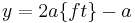$y=2a\{ft\}-a\,$	$a \over \sqrt 3$
Triangle wave	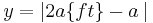$y=\|2a\{ft\}-a\,\|$	$a \over \sqrt 3$
Pulse train	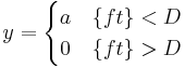$y=\begin{cases}a & \{ft\} < D \\ 0 & \{ft\} > D \end{cases}$	$a \sqrt{D}$
Notes: t is time f is frequency a is amplitude (peak value) D is the duty cycle or the percent(%) spent high of the period (1/f) {r} is the fractional part of r

Complex wave forms made from common known wave forms have a RMS that is the root of the sum of squares of the component RMS values, if the component waveforms are orthogonal (that is, if the average of the product of one simple waveform with another is zero for all pairs other than a waveform times itself).

$RMS_{Total} = \sqrt {{{RMS_1}^2 %2B {RMS_2}^2 %2B \cdots %2B {RMS_n}^2} }$

Uses

The RMS value of a function is often used in physics and electrical engineering.

Average electrical power

Electrical engineers often need to know the power, $P$ , dissipated by an electrical resistance, $R$ . It is easy to do the calculation when there is a constant current, $I$ , through the resistance. For a load of $R$ ohms, power is defined simply as:

$P = I^2 R.\,\!$

However, if the current is a time-varying function, $I(t)$ , this formula must be extended to reflect the fact that the current (and thus the instantaneous power) is varying over time. If the function is periodic (such as household AC power), it is nonetheless still meaningful to talk about the average power dissipated over time, which we calculate by taking the simple average of the power at each instant in the waveform or, equivalently, the squared current. That is,

$P_\mathrm{avg}\,\!$	$= \langle I(t)^2R \rangle \,\!$ (where $\langle \ldots \rangle$ denotes the mean of a function)
	$= R\langle I(t)^2 \rangle\,\!$ (as R does not vary over time, it can be factored out)
	$= (I_\mathrm{RMS})^2R\,\!$ (by definition of RMS)

So, the RMS value, $I_\mathrm{RMS}$ , of the function $I(t)$ is the constant signal that yields the same power dissipation as the time-averaged power dissipation of the current $I(t)$ .

We can also show by the same method that for a time-varying voltage, $V(t)$ , with RMS value $V_\mathrm{RMS}$ ,

$P_\mathrm{avg} = {(V_\mathrm{RMS})^2\over R}.\,\!$

This equation can be used for any periodic waveform, such as a sinusoidal or sawtooth waveform, allowing us to calculate the mean power delivered into a specified load.

By taking the square root of both these equations and multiplying them together, we get the equation

$P_\mathrm{avg} = V_\mathrm{RMS}I_\mathrm{RMS}.\,\!$

Both derivations depend on voltage and current being proportional (i.e., the load, R, is purely resistive). Reactive loads (i.e., loads capable of not just dissipating energy but also storing it) are discussed under the topic of AC power.

In the common case of alternating current when $I(t)$ is a sinusoidal current, as is approximately true for mains power, the RMS value is easy to calculate from the continuous case equation above. If we define $I_{\mathrm{p}}$ to be the peak current, then:

$I_{\mathrm{RMS}} = \sqrt {{1 \over {T_2-T_1}} {\int_{T_1}^{T_2} {(I_\mathrm{p}\sin(\omega t)}\, })^2 dt}.\,\!$

where t is time and ω is the angular frequency (ω = 2π/T, whereT is the period of the wave).

Since $I_{\mathrm{p}}$ is a positive constant:

$I_{\mathrm{RMS}} = I_\mathrm{p}\sqrt {{1 \over {T_2-T_1}} {\int_{T_1}^{T_2} {\sin^2(\omega t)}\, dt}}.$

Using a trigonometric identity to eliminate squaring of trig function:

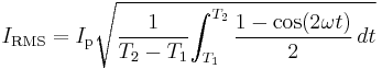
$I_{\mathrm{RMS}} = I_\mathrm{p}\sqrt {{1 \over {T_2-T_1}} {\int_{T_1}^{T_2} {{1 - \cos(2\omega t) \over 2}}\, dt}}$

$I_{\mathrm{RMS}} = I_\mathrm{p}\sqrt {{1 \over {T_2-T_1}} \left [ {{t \over 2} -{ \sin(2\omega t) \over 4\omega}} \right ]_{T_1}^{T_2} }$

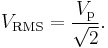
but since the interval is a whole number of complete cycles (per definition of RMS), the $\sin$ terms will cancel out, leaving:

$I_{\mathrm{RMS}} = I_\mathrm{p}\sqrt {{1 \over {T_2-T_1}} \left [ {{t \over 2}} \right ]_{T_1}^{T_2} } = I_\mathrm{p}\sqrt {{1 \over {T_2-T_1}} {{{T_2-T_1} \over 2}} } = {I_\mathrm{p} \over {\sqrt 2}}.$

A similar analysis leads to the analogous equation for sinusoidal voltage:

$V_{\mathrm{RMS}} = {V_\mathrm{p} \over {\sqrt 2}}.$

Where $I_{\mathrm{P}}$ represents the peak current and $V_{\mathrm{P}}$ represents the peak voltage. It bears repeating that these two solutions are for a sinusoidal wave only.

Because of their usefulness in carrying out power calculations, listed voltages for power outlets, e.g. 120 V (USA) or 230 V (Europe), are almost always quoted in RMS values, and not peak values. Peak values can be calculated from RMS values from the above formula, which implies V_p = V_RMS × √2, assuming the source is a pure sine wave. Thus the peak value of the mains voltage in the USA is about 120 × √2, or about 170 volts. The peak-to-peak voltage, being twice this, is about 340 volts. A similar calculation indicates that the peak-to-peak mains voltage in Europe is about 650 volts.

It is also possible to calculate the RMS power of a signal. By analogy with RMS voltage and RMS current, RMS power is the square root of the mean of the square of the power over some specified time period. This quantity, which would be expressed in units of watts (RMS), has no physical significance. However, the term "RMS power" is sometimes used in the audio industry as a synonym for "mean power" or "average power". For a discussion of audio power measurements and their shortcomings, see Audio power.

Amplifier power efficiency

The electrical efficiency of an electronic amplifier is the ratio of mean output power to mean input power. The efficiency of amplifiers is of interest when the energy used is significant, as in high-power amplifiers, or when the power-supply is taken from a battery, as in a transistor-radio.

Efficiency is normally measured under steady-state conditions with a sinusoidal current delivered to a resistive load. The power output is the product of the measured voltage and current (both RMS) delivered to the load. The input power is the power delivered by the DC supply, i.e. the supply voltage multiplied by the supply current. The efficiency is then the output power divided by the input power, and it is always a number less than 1, or, in percentages, less than 100. A good radio frequency power amplifier can achieve an efficiency of 60–80%.^[2]

Other definitions of efficiency are possible for time-varying signals. As discussed, if the output is resistive, the mean output power can be found using the RMS values of output current and voltage signals. However, the mean value of the current should be used to calculate the input power. That is, the power delivered by the amplifier supplied by constant voltage $V_{CC}$ is

$P_\mathrm{input}(t) = I_Q V_{CC} %2B I_\mathrm{out}(t) V_{CC}\,$

where $I_Q$ is the amplifier's operating current. Clearly, because $V_{CC}$ is constant, the time average of $P_\mathrm{input}$ depends on the time average value of $I_\mathrm{out}$ and not its RMS value. That is,

$\langle P_\mathrm{input}(t) \rangle = I_Q V_{CC} %2B \langle I_\mathrm{out}(t) \rangle V_{CC}.\,$

Root-mean-square speed

Main article: Root-mean-square speed

In the physics of gas molecules, the root-mean-square speed is defined as the square root of the average speed-squared. The RMS speed of an ideal gas is calculated using the following equation:

${v_\mathrm{RMS}} = {\sqrt{3RT \over {M}}}$

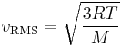
where $R$ represents the ideal gas constant, 8.314 J/(mol·K), $T$ is the temperature of the gas in kelvins, and $M$ is the molar mass of the gas in kilograms. The generally accepted terminology for speed as compared to velocity is that the former is the scalar magnitude of the latter. Therefore, although the average speed is between zero and the RMS speed, the average velocity for a stationary gas is zero.

Root-mean-square error

Main article: Root-mean-square error

When two data sets—one set from theoretical prediction and the other from actual measurement of some physical variable, for instance—are compared, the RMS of the pairwise differences of the two data sets can serve as a measure how far on average the error is from 0.

The mean of the pairwise differences does not measure the variability of the difference, and the variability as indicated by the standard deviation is around the mean instead of 0. Therefore, the RMS of the differences is a meaningful measure of the error.

RMS in frequency domain

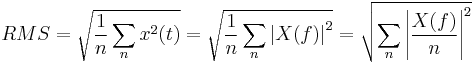
The RMS can be computed also in frequency domain. The Parseval's theorem is used. For sampled signal:

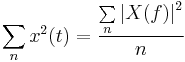$\sum\limits_{n}{{{x}^{2}}(t)}=\frac{\sum\limits_{n}{{{\left| X(f) \right|}^{2}}}}{n}$ , where $X(f)=FFT\{x(t)\}$ , $n$ is number of $x(t)$ samples.

In this case, the RMS computed in time domain is the same as in frequency domain:

$RMS =\sqrt{\frac{1}{n}\sum\limits_{n}{{{x}^{2}}(t)}} = \sqrt{\frac{1}{n}\sum\limits_{n}{{{\left| X(f) \right|}^{2}}}} = \sqrt{\sum\limits_{n}{{{ \left|\frac{X(f)}{n}\right| ^ 2 }}}}$

Relationship to the arithmetic mean and the standard deviation

If $\bar{x}$ is the arithmetic mean and $\sigma_{x}$ is the standard deviation of a population or a waveform then:^[3]

$x_{\mathrm{rms}}^2 = \bar{x}^2 %2B \sigma_{x}^2.$

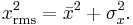
From this it is clear that the RMS value is always greater than or equal to the average, in that the RMS includes the "error" / square deviation as well.

Physical scientists often use the term "root mean square" as a synonym for standard deviation when referring to the square root of the mean squared deviation of a signal from a given baseline or fit. This is useful for electrical engineers in calculating the "AC only" RMS of a signal. Standard deviation being the root mean square of a signal's variation about the mean, rather than about 0, the DC component is removed (i.e. RMS(signal) = Stdev(signal) if the mean signal is 0).

References

^ Cartwright, Kenneth V (Fall 2007). "Determining the Effective or RMS Voltage of Various Waveforms without Calculus". Technology Interface 8 (1): 20 pages. http://technologyinterface.nmsu.edu/Fall07/
^ Terman, F.E. (1955) Electronic and Radio Engineering, McGraw Hill, New York
^ Chris C. Bissell and David A. Chapman (1992). Digital signal transmission (2nd ed.). Cambridge University Press. p. 64. ISBN 9780521425575. http://books.google.com/books?id=ItJoq36hCoYC&pg=PA64.